DOI: 10.31038/NRFSJ.2022522
Abstract
Respondents from three countries (France, Germany, and UK) each evaluated unique sets of 60 vignettes about coffee, created by combining elements (messages) according to an underlying experimental design. Respondents rated each vignette on an anchored 9-point scale of craving (1=do not crave. 9=crave extremely). The ratings were deconstructed into individual level models, showing the contribution of each message to craveability. By incorporating an extensive self-profiling classification questionnaire, the research paradigm, Mind Genomics, revealed the nature of how respondents think about coffee, showing the contribution of the message itself, as well as the country, and the nature of what the respondent does in terms of coffee behavior. The paradigm presents the potential for a deep understanding of the mind of the ordinary person, doing ordinary tasks, e.g., those involved with coffee, and allows the affordable and easy creation of large-scale databases of human behavior and decision making.
Introduction
As this paper is being written the world of coffee is actively evolving. From a drink in a modern day ‘coffee house’ enjoyed in leisure, coffee has become what might well be the most popular beverage in the world, emblematic of different social norms around the world, and today a source of involvement in societal-moral issues. Coffee has evolved into a drink that people enjoy together in coffee houses, chatting, reading paper, starting their morning with a quick cup, or passing the day leisurely [1,2]. Moving further, coffee ready to drink comes in a variety of ‘forms’, whether traditional ‘black’, doctored up with all sorts of other ingredients [3,4]. Coffee has emblemized social change. During the past decades consumers have fallen in love with Italian espresso coffee, so much so that that one can feel an Italiphila (love of things Italian) pervading the word through the world-wide reception of espresso [5-7].
This most popular drink has, in turn, evolved into a topic of social concern. In, study after study the academic literature has started to focus on social issues, such as the environment as well as ‘fair trade’ for the farmers who grow the coffee beans [8-11]. The sheer popularity of coffee in daily life and the social significance of fair trade to pay the farmer the real value of the coffee make the topic irresistible to academics. Google® has 62,400 hits for the topic ‘coffee and fair trade’, Google Scholar® has about 8x as many, 481,000 hits for coffee and fair trade!
Despite the importance of coffee, there are relatively a handful of academic papers on the topic of coffee itself. Some of these are studies the sensory properties of coffee, and the different pattern of preferences for these sensory properties. For example, Geel et al. (2005) reported that four patterns of the acceptance emerging from the response to 11 coffees: “Based on consumer preferences, four consumer groups were identified, “pure coffee lovers” (23%), “coffee blend drinkers” (30%), “general coffee drinkers” (37%) and “not serious coffee drinkers” (10%). The “pure coffee lovers” prefer the more astringent, bitter, roasted, nutty and full-bodied flavour of the pure coffee samples. The less intense coffee flavour character, but higher sweetness and root flavour, typical of chicory blended instant coffee, were attributes that were preferred by the “coffee blend lovers”. The “general coffee drinkers” seem to consume coffee out of habit and are less concerned about the specific sensory properties of the coffee [12].”
The academic literature is equally sparse when it comes to what to communicate about coffee in order to entice prospective buyers. From the author’s own experience, the companies selling coffee do extensive research, from basic attitudes and usage studies (A&U) dealing with coffee as part of life, and then concept tests to find out the acceptance of new ideas, and finally advertising evaluation to find out ‘what works’.
One might think that the knowledge is extensive in corporations about the aspects of coffee, specifically the most persuasive messaging. The author’s experience, however, over the past 46 years since 1976 would suggest just the opposite. There seems to be no systematic study about coffee messaging that the author has ever encountered in the public literature, nor has the author encountered evidence of this systematic approach in private consulting. There are tests of individual messages, but no large scale, systematic tests of the mind of the coffee consumer regarding the language of coffee. When directly confronted with the request ‘show me the book of messages which work with consumers’ no one, either in academia or in business has been ever able to provide the request ‘book’ or at least ‘database.’
Getting into the Mind of the Coffee Consumer through Mind Genomics
Given the importance of coffee, there is an extraordinarily amount known about the consumer attitudes towards coffee and the consumption patterns of the actual product, most of the information residing in the file cabinets and stored and archived ‘banker’s boxes’ of study results owned by corporations usually residing in dead storage. Indeed, the author’s own experience with Maxwell House Division of General Foods Corporation in the mid 1980’s suggested that for General Foods Corporation alone, the consumer research budget was in the millions of dollars, with hundreds of reports issued by the market research department as well as by the sensory evaluation department. What new, if anything, can consumer-focused scientific research add with to what has been developed with the large corporate budgets? Can we learn new things about the way people think about coffee?
Despite the richness of information, from the public domain (popular press, from companies, and from presumably more objective science there still is a lot to be discovered, which is where the emerging science of Mind Genomics enters. Mind Genomics was developed from a different world view, that of looking at how people make decisions when confronted with compound stimuli, mixtures of messages, the more typical situation in nature. Mind Genomics traces its heritage to conjoint measurement [13] and to experimental design [14].
Mind Genomics paints word pictures of products (and intangibles, such as service), these word pictures created from defined combinations of simple phrases that a person would encounter during everyday experience. The combinations are called ‘vignettes.’ Using statistical methods such as OLS (ordinary least-squares) regression to deconstruct the response to the mixture into the driving power of the components, viz., elements. Mind Genomics studies ends up being far deeper, and often far more ‘actionable’ for science and business purposes than information and ‘insights’ emerging from conventional qualitative, quantitative, and behavioral studies [15,16].
The foregoing approach of mix/evaluate/deconstruct is quite different from that used in conventional research, where the respondent is presented with one idea or question after another, forced to focus on an array of topics which keep changing. In such a system, viz. the typical questionnaire, the respondent must keep changing her or his frame of reference, first thinking for example about the occasion, and then about the product, and then about feelings, etc.
It! Studies – the Lure of Mind Genomics Databases across Products and Across Countries
After successful research with Mind Genomics in the world of foods, the McCormick & Company approached the author and colleague Jacqueline Beckley of the Understanding and Insight Group, Inc. to extend the scope of Mind Genomics studies that they had already run. Rather than applying Mind Genomics to one topic of food, the research sponsor at McCormick, Director Dr. Hamed Faridi, wanted to look at a whole set of foods, the elements appropriate for that food, but with common elements dealing with emotion benefits. This effort become the 2001 Crave It! study, a study of 30 foods then repeated with teens, rather than with adults [17]. The study was massive by any consideration, with each study comprising more than 100 respondents, and exactly 36 elements, combined into unique sets of 60 vignettes for each respondent. The results were analyzed ‘globally’ to identify recurring themes among people. The data suggested that across all the 30 studies, three patterns continued to emerge: Elaborates, Imaginers, and Classics. These groups, so-called ‘mindsets’ clearly differed in terms of the particular elements which appealed to them. The Elaborates focuses on the food, the Imaginers on the situation, and the Traditionals on the typical factors involved with the food, such as enjoyment, price, etc.
About a year later, the same idea was supported by the Firmenich Corporation, this time looking at foods in three western European countries, France, Germany and the UK, respectively. The structure was the same, and at that time the focus was on the re-emergence of the three now ‘canonical’ groups of respondents, again based upon the pattern of their coefficients when the data from each country and each food were more deeply analyzed [18]. Nothing of the sort had been done before. The notion was conceived of and developed by Pieter Aarts of Belgium, Klaus Paulus of Germany, and the It! Ventures LLC in the US (Jacqueline Beckley and Howard Moskowitz). The studies, sponsored by Firmenich in Switzerland, were designed to understand how people respond to different ideas and descriptions of food, not so much using the traditional attitude and usage sales, but rather using the new method of experimentation offered by Mind Genomics.
The Eurocrave Studies on Coffee
The three studies reported here come from the early days of Mind Genomics, when getting respondents showed that respondents could participate with little difficult, as long as they were somewhat motivated. During the early years of this century the novelty of the Internet was such that people were intrigued. The respondents were sent invitations, and offered a chance to participate in a sweepstakes for money. This sufficed to bring in thousands of respondents, these thousands choosing to participate in a study that interested them.
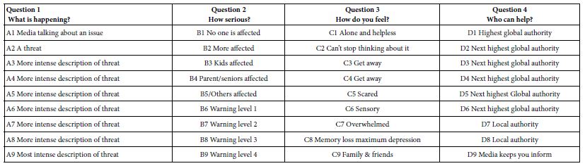
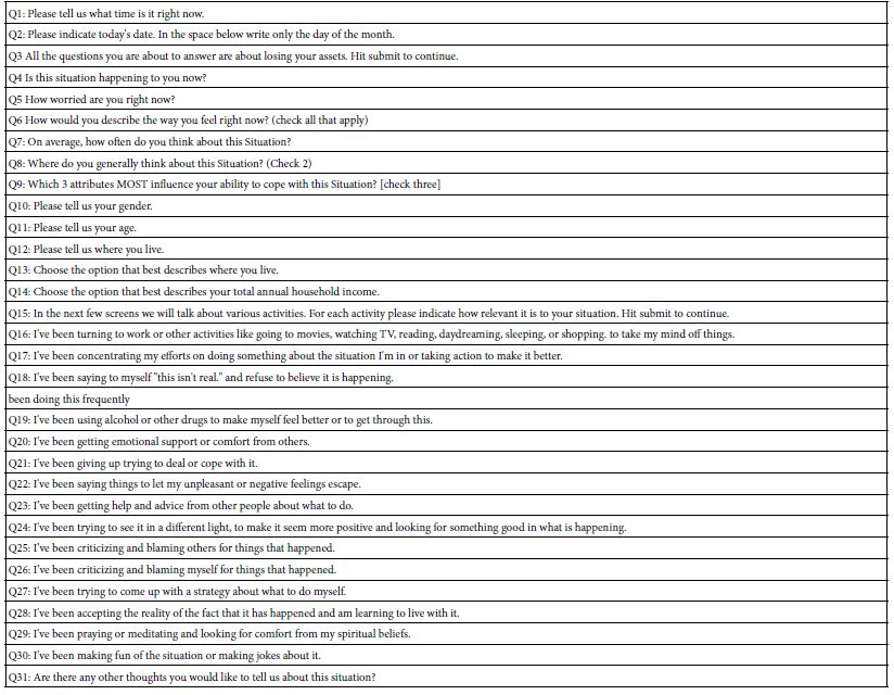
The actual Mind Genomics study, positioned as a ‘survey’, was actually an experiment. The word ‘experiment’ is negatively tinged, but the word survey and the word opinion is not. The Mind Genomics approach begins with a topic, requires a set of four questions, and nine answers to each question. The questions tell a story, or provide distinct types of information. These early studies, of which Crave It! and Eurocrave! are examples, show the early focus on acquiring as much information as possible about a topic?
The ingoing notion of Mind Genomics was and remains the idea that we can learn a lot by presenting a person with combinations of messages, and instruct the respondent to rate the combination. Rather than polishing the combination so the combination becomes a dense paragraph, albeit a well-written one, the Mind Genomics experiments virtually ‘throws’ the ideas at the respondent, instructing the respond to react to the combination. The approach is a bit off-putting at first, because respondents are far more accustomed to well written, dense paragraphs. An analogy is the difference between a compote comprising many fruits versus a thrown-together fruit salad.
The structure required four questions, each with nine answers. The objective of the experimental design was to ensure that the elements would be put together in such a way that each vignette would have at most one answer from two, three, or four questions. The actual design, four questions by nine answers per question, is a template, required for ‘bookkeeping’, so that a vignette would never have two answers from a single question, answers that might contradict each other.
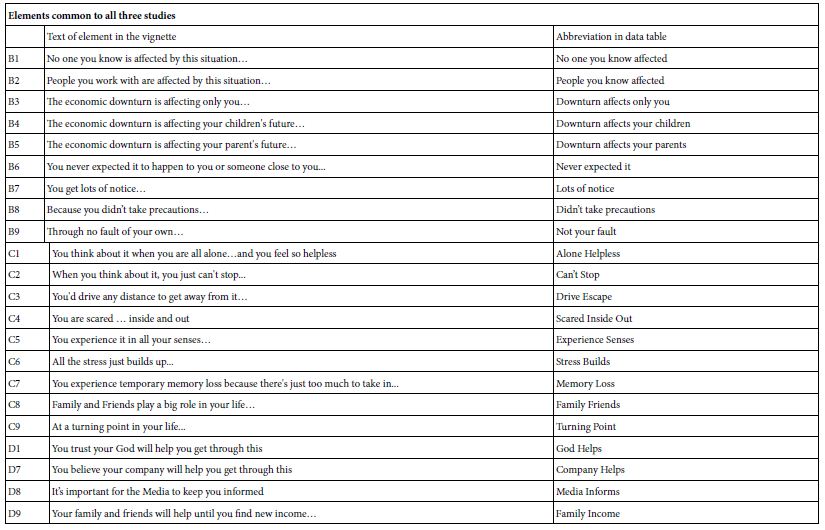
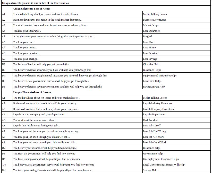
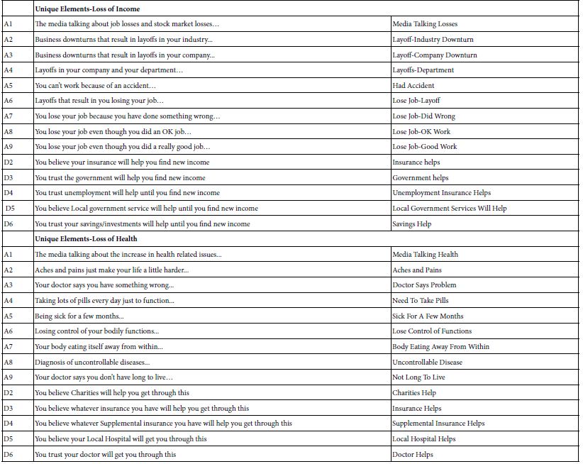
Table 1 shows the raw materials, the elements, from the three studies, one in the UK, one in France, and one in Germany. The elements are in the native language. As much as possible the elements were the same across countries, but that equivalence of elements was not possible in the case of brands or stores present in one country but not in the other. Table 1 shows that the same idea might be expressed in slightly different ways by country. Thus, one should look at the elements as specific instantiations of more general ideas, instantiations which may differ across countries. This caveat means that the data should not be rigorously compared across countries, simply because the execution of the same idea in one country might be quite different from the execution of the same idea in another country.
Table 1: Elements for the three-country Eurocrave study on coffee
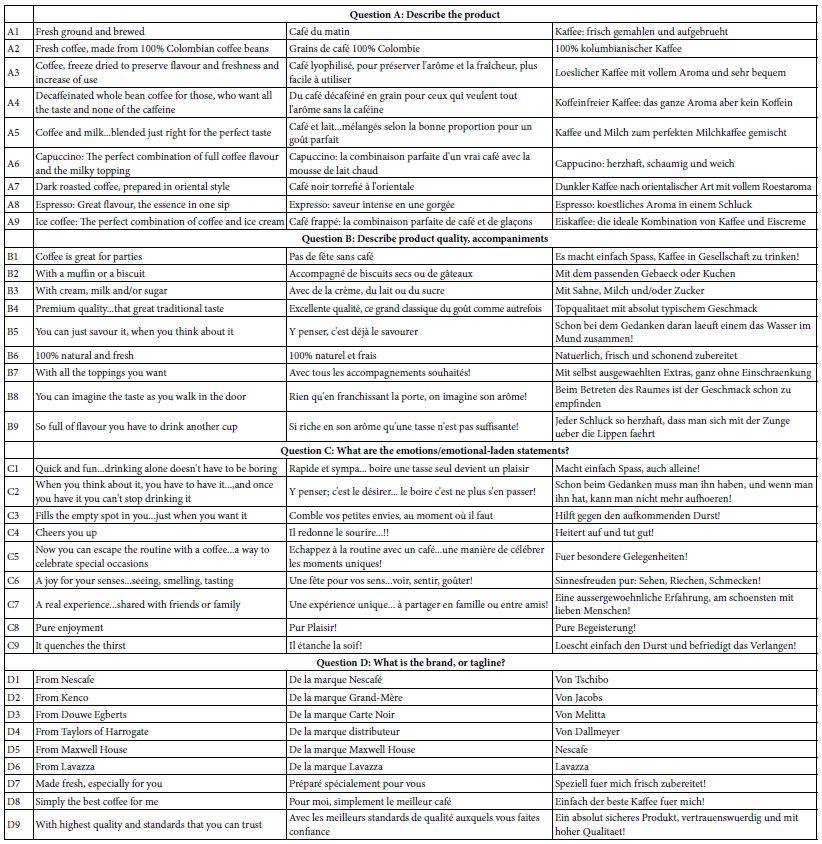
One of the hallmarks of Mind Genomics is the use of language that is best characterized as ‘colloquial.’ That is, the elements themselves are phrased in the way a person of the country might talk. In the actual Mind Genomics experiment this effort to be simple and colloquial will end up playing an important role. The language itself will allow the respondent to ‘graze’ through the text, rather than force the respondent to think about the answer. That is, the simple declarative format will simplify the respondents task, with the respondent simply looking at easy-to-understand sets of phrases.
Running the Mind Genomics Experiment
In conventional studies, specifically surveys, the study is set up so that the respondent must focus on a single question, answer it, and then move on to the next. The effort is made to minimize respondent bias although it is in the nature of respondents to want to please the researcher, and to give the correct answer Whether the respondent can actually come up with the ‘correct answer’ is not important. What is important is the pervasive subconscious nature to be right or at least to be consistent. Such biases abound in survey research. Researchers attempt to counteract these biases by such strategies as rotating the order questions in order to reduce effects due to test order, and disguise the nature of the topic so that that the respondent cannot really guess about the goal of the question.
The Mind Genomics approach to the interview is described as a survey to people, but as stated above, the reality is that Mind Genomics constitutes really a well -controlled experiment. The experimenter presents test stimuli (viz., combinations of messages, the aforementioned elements shown in Table 1), obtains a response (a rating of the vignette by the respondent), repeats the task, collects the data, and then relates the presence/absence of the elements to the ratings. The respondent simply rates the combination, almost it would appear from exit interview, assigning the ratings in what is report as a guessing, or in a state of indifference because the task seems daunting.
The respondent in the Mind Genomics experiments does not evaluate one phrase at a time, viz., rate 36 phrases. Rather, the respondent in a study is exposed to 60 different combinations of these elements, each combination comprising 2-4 elements, no more than one element or answer from a question. The respondent is simply instructed to the read the vignette (combination of elements) as one idea, and rate the combination on a nine-point scale. The scale is simple, anchored at both ends:
Using this 9-point scale, please show how you feel about the COFFEE as described:
1 = Do not crave it at all … 9= Definitely crave it
Most people participating in the study, or even just inspecting the set of 60 vignettes, the combinations of elements, feel that the elements have been thrown together randomly. Nothing could be further from the truth. The underlying structure for the 60 combinations is dictated precisely by an experimental design, a blueprint, which defines the specific elements present in each combination.
The experimental design provides these convenient features and benefits:
- Each vignette comprises a specific set of elements. The minimum number of elements is two, the maximum number is four. By design, many of the vignettes are incomplete. Each element appears equally often, five times in 60 vignettes, and absent 55 times from the 60 vignettes. Doing the arithmetic shows that each of the four questions contributes 45 elements to the 60 vignettes and is absent from the remaining 15 of the 60 vignettes.
- No vignette comprises more than one element (answer) from a specific question. The underlying rationale is that no vignette can carry mutually contradictory information of the same type (e.g., no vignette can comprise two brands).
- Each respondent tests a unique set of 60 vignettes, different from the 60 vignettes tested by any other respondent. This approach, permuted designs, was patented by author Moskowitz and colleague Alex Gofman [19].
- The happy outcome of the structure is that one can create an equation relating the presence/absence of the 36 elements to the rating (or a transform of the rating), at the level of a single respondent, or at the level of a group of respondents. This ‘within subjects’ feature allows clustering algorithms to identify groups of respondents with similar patterns of coefficients, viz., ‘mind-sets’ in the language of Mind Genomics [20].
The studies for Eurocrave were set up in the United States. Local field services in the three countries invited respondents to participate by internet survey. The respondent was invited to participate by the local field service in the country, a field service with a specialty in recruiting panelists for web-based, viz. online, studies.
It is important to keep in mind that even as far back as 2002, two decades ago, it was virtually impossible to source a sufficient number of respondents from one’s friends and colleagues. The notion that people want to participate in research interviews, whether with live interviewers or on the web, is simple unreasonable, then, and increasingly so. One cannot expect people to offer their time for free. It is important to compensate them, and even more important to work with companies specializing in providing people to participate in consumer research studies. The criticism that these may become ‘professional respondents’ is far less cogent than the almost certain fact that depending upon the goodwill of random people, even students in a class, will probably end up with fewer respondents than needed.
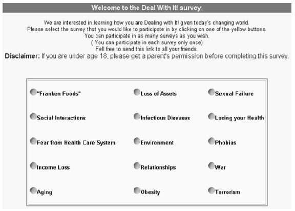
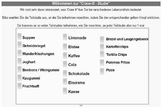
Each of the three countries had a pre-created ‘wall’ listing the different foods being covered in the Eurocrave project. Figure 1 shows the wall for the German study. The wall was designed with three properties in mind.

Figure 1: The wall for the Eurocrave study (Germany)
- The studies (really names of the foods) appeared in random order, to minimize the selection of studies in one position, e.g., the top right.
- When a study had 120 respondents who successfully completed the study, the study temporarily ‘disappeared’ from the wall, so it could not be chosen. The respondent had to choose from among the less popular studies.
- The happy consequence of this strategy was that respondents only participated in a study, which interested them.
The respondent was led to the correct study, read the introduction informing the respondent of the topic and the length of time (15 minute), and then presented the respondent with the vignettes, one after another. As soon as the respondent pressed the rating key the vignette disappeared, and the next vignette appeared in its place. There was no opportunity to change the rating once it was assigned. Afterwards, the respondent completed a self-profiling questionnaire dealing with different aspects of who the respondent IS, what the respondent THINKS regarding coffee, as well as the time of day that the respondent was completing the study.
Strategy for Analysis and for Presentation of Results
Most users of data do not feel comfortable with Likert scales, like the scale for craveability. They do not know what the scale means, even though respondents seem to have no trouble using the scale, AND the scale allows for valid statistical analysis.
Many researchers feel that they learn more when they can divide the scale into two parts, viz. NO and YES, respectively. It is easier for managers to understand NO vs YES. To make the research easier to understand, the data were divided into two points, ratings 1-6 transformed to 0, ratings 7-9 transformed to 100. This division was arbitrary but made intuitive sense. After the foregoing transformation, a vanishingly small random number was added to each transformed value, so that the ratings were slightly different from 0 or 100, and slightly different from each other when they had been transformed. This addition of the small random number enabled the dependent variable for each respondent to show some variation across vignettes, even when the respondent confined her or his ratings to the lower part of the scale (1-6, always transformed to 0) or to the upper part of the scale (7-9 always transformed to 100). The variation ensured the data be further processed at the level of the individual respondent.
The individual data were analyzed by OLS (ordinary least-squares) regression, which estimated the additive constant (k0) and the 36 coefficients (k1-k36), one coefficient for elements A1-D9, respectively. The regression equation is expressed as: Transformed Rating = k0 + k1(A1) + k2(A2) …. K36(D9).
The regression equation summarizes the data for a respondent or group of respondents. The additive constant, k0, can be interpreted ais the estimated proportion of respondents who would rate a vignette 7, 8 or 9, respectively, in the absence of elements. Of course, the underlying experimental design ensures that no vignette will comprise fewer than two elements, so the additive constant is a purely estimated parameter. The additive constant plays a role, becoming a baseline value of the likelihood of respondent assigning a positive rating of 7, 8 or 9. High additive constants (e.g., 50 or more) mean that the respondent has a predilection for up-rating vignettes. In this ‘happy’ situation, a vignette simply has to feature elements which are slightly positive, and avoid elements which are negative. Low additive constants (e.g., lower than 30, for example) mean that for a vignette to get a high rating of 7, 8 or 9, respectively, the elements ought to be strong performers because the predilection of the respondent is to use the lower part of the scale.
The analysis of the ratings by OLS regression produces a large data set, namely 37 numbers for each respondent. The 37 numbers per respondent is far smaller than the matrix required to code the raw data for the respondent. The original data for each respondent constituted requires 60 rows of numbers, beginning with information about who the respondent is, what the respondent does, et., continuing then into 36 columns (one column for each element), then the rating, and then the transformed rating. This matrix contains one row per vignette per respondent. Across all 60 rows for a single respondent the information about the respondent remains the same, but the data fields corresponding to the structure of the vignette (which element appear, which do not appear), and the rating, change from vignette to vignette.
The Mind Genomics exercise produces a great deal of data, specifically 37 numbers per subgroup of respondents. It is impractical and counterproductive to report the data from each element across all of the relevant subgroups (viz. total panel and key self-defined subgroups, as well as emergent mind-sets). The amount of data for one subgroup overwhelms. Multiply that amount of information by the number of subgroups relevant to an analysis, and one can easily end up with 100+ cells of data. Looking for a pattern across 100 cells is data is simply too difficult.
One of the ways to cut down on the amount of data, and allow important data through, is to eliminate any coefficient less than a certain value for any of the 36 elements. The standard error of the coefficient is 4-5 for these studies, so a coefficient of 8 or 9 is likely to be significant, and more important, likely to signify something relevant about the topic. Thus, a coefficient of 10 or higher can be considered important. Other coefficients, viz., those below 10, need not be shown, and thus allowing the patterns to emerge. For this paper we will only look at coefficients of +10 or higher. As we begin the analysis of the data, it will quickly become apparent that most of the elements do not have strong performing coefficients, simplifying our search for patterns. Furthermore, each data table will show highlighted elements, viz., elements which score well (coefficient of 10 or higher) for at least three subgroups. These are ‘strong performers,’ viz., ‘strong performing elements.
Results
Who the Person Is – Total and Gender
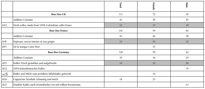
We begin the analysis with the total panel and with males and females (Table 2). The first analysis looks at the additive constant. Recall that the additive constant is a baseline, or at least can be interpreted as a baseline. Looking at Table 2, we see that the additive constants differ by country. Those for the UK and France are 41, moderate, but the elements show low coefficients. The additive constant for Germany is low, 30, but more elements are strong performers.
Table 2: Strong performing elements for total panel and for gender
From study after study one of four patterns emerge, to describe the value of the additive constant and the value of the coefficients:
- Low additive constant, low values for the coefficients – an unpopular idea. A good example is credit cards. The values of the additive constant are usually 0 or even negative up to about 20.
- Moderate additive constant, low values for the coefficients. The value for the additive constant is 20-50. Here the basic idea is neutral, buoyed up by some good ideas if any.
- Moderate additive constant, high values for many coefficients. The value for the additive constant is again 20-50-. Here the basic idea is neutral Here the respondent is discriminating among the elements, with some elements really being winners.
- High additive constant, low values for many coefficients. The value for the additive constant is 50 or higher. Here the basic idea is very good, and the respondent does not really find elements to strongly augment the already-high basic response to the vignette.
The second analysis looks at the strong performing elements. Surprisingly, the three countries exhibit few strong performing elements, at least for total sample and gender. Respondents in each country show only one strong performing element each across all three groups (total, two genders). The elements are different, but all from Question or Group A, dealing with the description of the product itself. This finding surprises because of the absence of strong-performing elements, but is in line with other studies from Mind Genomics which point to the importance of an appetizing description of the product as a driver of strong performance.
UK: AE2 Fresh coffee, made from 100% Colombian coffee beans
France: AF8 Expresso: saveur intense en une gorgée
Germany: AG1 Kaffee: frisch gemahlen und aufgebrueht
Who the People Are – Age
The self-profiling classification allowed the respondent to report their age. Table 3 shows age does not play an important role. The additive constants show a mixed pattern, increasing with age in the UK, decreasing with age in France (except for a very low additive constant for those 18-25), and not clear in Germany, which presented only two ages.
Table 3: Strong performing ‘coffee elements’ for three countries, by age
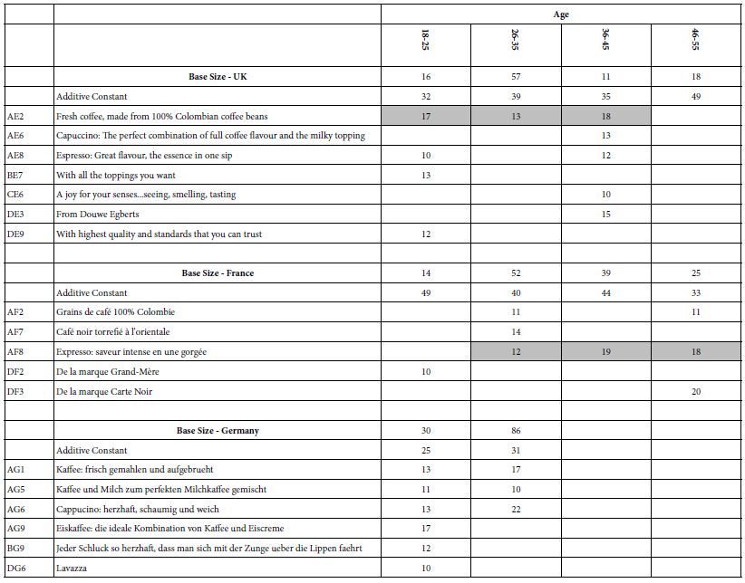
The strong elements in country are different, but again it is important to note that the strongest elements come from the first group of elements, the first question, about the product.
UK: AE2 Fresh coffee, made from 100% Colombian coffee beans
France: AF8 Expresso: saveur intense en une gorgée
When the Respondent Participated – Time of Day
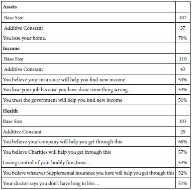
One of the foci of the It! studies, such as our coffee study, was the question regarding differences in the additive constant and in the coefficients. Table 4 shows the relevant data.
These patterns emerge:
- The additive constants are almost all quite low. It is the elements which must do the work.
- The additive constants increase from morning to night, suggesting a more positive ‘basic response’ to the message at night. The pattern is not perfect, however, but is worth noting because there may be an increasing sensibility about the quality of the coffee as the day progresses, with the quality of the coffee less important than the ability to ‘wake one up’, expected to be the case in the morning hours.
- The only time which does not feature many very strong performing elements is 6pm to 9pm.
- UK respondents do not show strong performing elements emerging in the three hour period of 9PM to 12 Midnight, whereas in contrast, French and German respondents do.
- The strong performing elements are:
Table 4: Strong performing ‘coffee elements’ for three countries, by daypart (three hour segments)
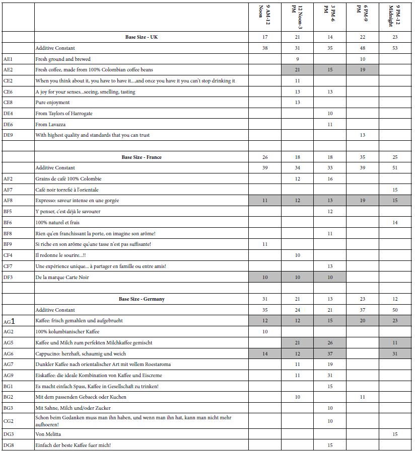
UK: AE2 Fresh coffee, made from 100% Colombian coffee beans
France: AF8 Expresso: saveur intense en une gorgée
DF3 De la marque Carte Noir
Germany: AG6 Cappucino: herzhaft, schaumig und weich
AG1 Kaffee: frisch gemahlen und aufgebrueht
AG5 Kaffee und Milch zum perfekten Milchkaffee gemischt
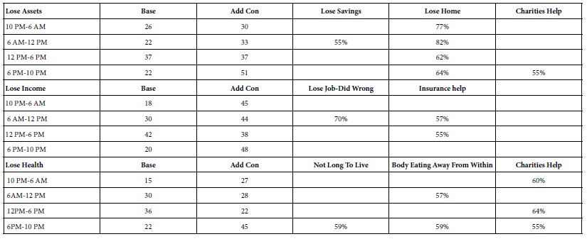
How the Respondent Felt – Self-Reported Thirst
As part of the self-profiling questionnaire the respondent selected the level of thirst experienced. Once again across the three countries on a few elements perform well for different levels of perceived thirst (Table 5)
Table 5: Strong performing ‘coffee elements’ for three countries, by self-reported degree of thirst
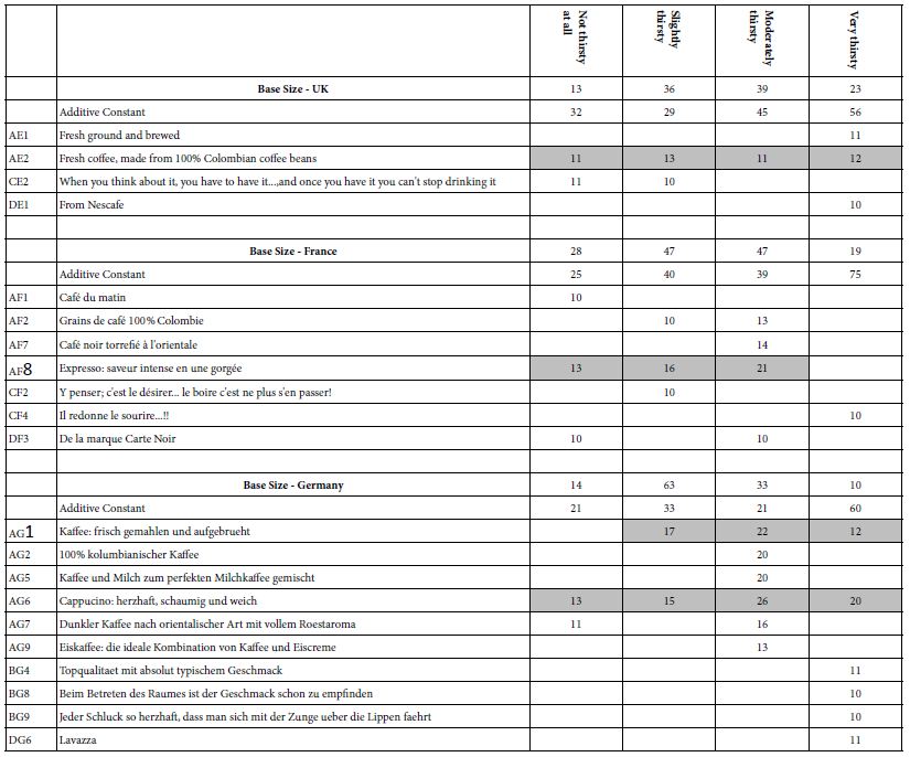
There are two patterns here worth noting:
- The additive constant is much higher when the respondent reports a high degree of thirst
- All strong performing elements showing up in three or more states of thirst come from Question A, dealing with product.
UK: AE2 Fresh coffee, made from 100% Colombian coffee beans
France: AF8 Expresso: saveur intense en une gorgée
Germany: AG6 Cappucino: herzhaft, schaumig und weich
AG1 Kaffee: frisch gemahlen und aufgebrueht
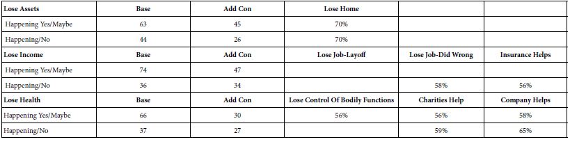
Coffee Behavior – Frequency of Coffee Consumption
Table 6 shows that the vast majority of respondents participating in this study were frequent coffee drinkers. One of the more interesting things emerging from Table 6 is that those who drink coffee less frequently, viz., once a day, find more evocative elements of interest.
Table 6: Strong performing ‘coffee elements’ for three countries, by self-reported frequency of drinking coffee
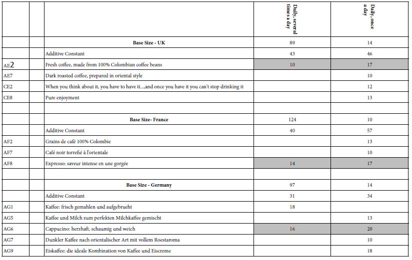
UK: AE2 Fresh coffee, made from 100% Colombian coffee beans
France: AF8 Expresso: saveur intense en une gorgée
Germany: AG6 Cappucino: herzhaft, schaumig und weich
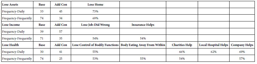
Coffee Behavior – Day-part of Coffee Consumption
Depending upon one’s culture, coffee can be consumed any time during the day or night. It is only a matter of cultural norms and one’s predilections. Table 7 shows that the most frequent day-part differs by country. Looking at the frequency of 30 respondents or more we find the following:
Table 7: Strong performing ‘coffee elements’ for three countries, by self-reported time of day when coffee is consumed
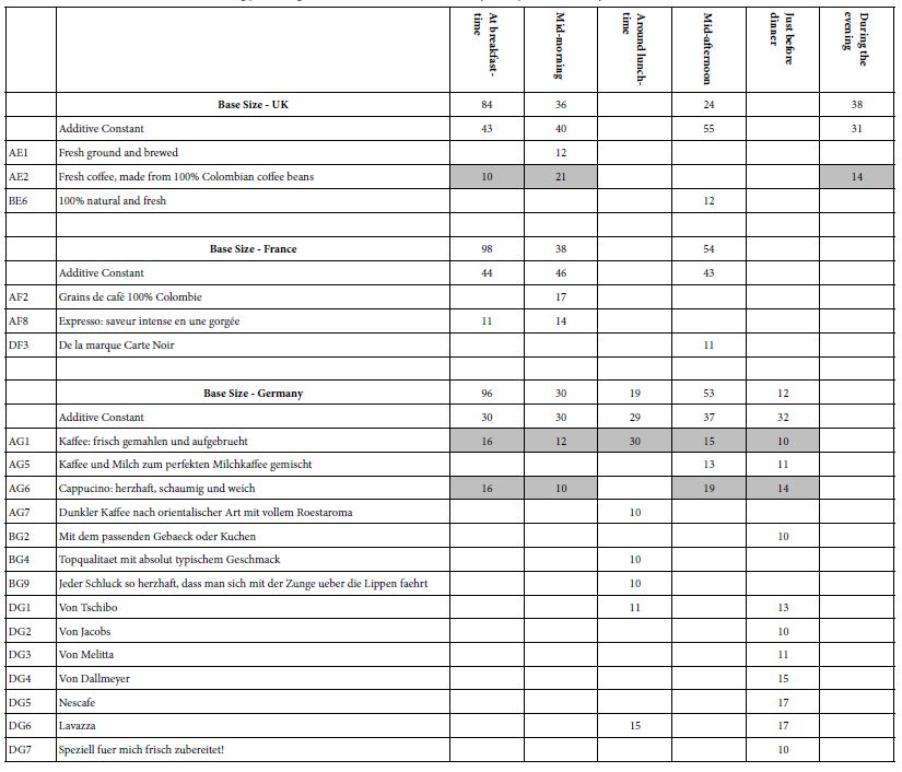
UK – breakfast most, and then evening and finally mid-morning parts. Highest additive constant in the mid-afternoon, lowest in the evening.
AE2 – Fresh coffee, made from 100% Colombian coffee beans
France – breakfast most, then mid-afternoon, and finally mid-morning. French respondents do not say that they drink coffee in the afternoon. The same size additive constant for breakfast, mid-morning, and mid-afternoon, respectively.
Germany – breakfast most, then mid-afternoon, then mid-morning. The same additive constant across all times (from breakfast to just before dinner)
AG1 – Kaffee: frisch gemahlen und aufgebrueht
AG6 – Cappucino: herzhaft, schaumig und weich
The ‘bottom line’ is that there are dramatic differences across countries, and even differences in the performance of elements in a single country across dayparts. The patterns are difficult to summarize.
Coffee Behavior – Where Coffee is Purchased or Consumed
In the self-profiling questionnaire the respondents checked off the places where they purchase or consumed coffee. Table 8 shows the distribution of the responses across five venues. The venues are not equally represented across the three countries, however, primarily due to low base sizes of respondents.
Table 8: Strong performing ‘coffee elements’ for three countries, by self-reported venue of purchase or consumption
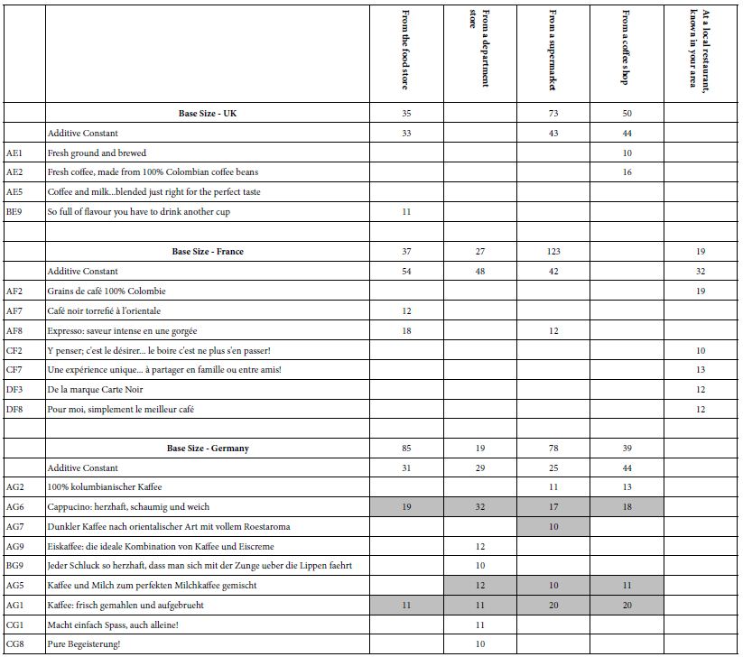
UK – Not in a department store nor in a local restaurant known in one’s area. The UK respondents purchase their coffee in a supermarket or food store. It may well be that the respondents don’t think of drinking coffee after a meal in a local restaurant as a real ‘coffee occasion’.
France – The French respondents purchase their coffee in a supermarket, and do think about coffee consumed in a local restaurant, but again without the strong focus of that as being a real ‘coffee occasion.’ (The base size is only 19 respondents). The French respondents consider coffee at a department store as a real coffee occasion.
Germany – The German respondents think of all venues (food store, department store, supermarket, coffee shop) as coffee occasions, but do not think of local restaurants and coffee as coffee occasions. German respondents show the greatest number of strong-performing elements associated with venue.
Coffee Attitudes – Features Selected as Important
The self-profiling classification questionnaire contained a question about what features of coffee the respondent felt to be important. The respondent could select up to three features. These features comprise, respectively, sensory aspects (appearance, aroma, taste), emotional aspects (memories, associations, brand), package features (packaging), and consumption features (portion size, social situation, mood).
Table 9 shows the patterns. As one would expect, aroma and taste, the sensory impressions, are chosen most frequently. The remaining features are distributed in different ways by country and show different patterns. In the interest of simplicity, we focus only on groups comprising 30 respondents or more.
Table 9: Strong performing ‘coffee elements’ for three countries, by self-reported selection of ‘what is important’
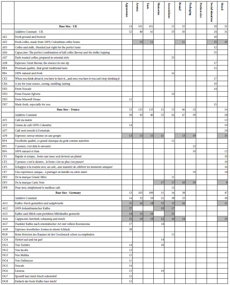
UK – Brand and mood are chosen most frequently.
Those choosing brand show a higher additive constant (50), but few strong performing elements. No brand elements are chosen!
Those choosing mood show a lower additive constant (31) and only two strong performing elements
France – Only brand chosen frequently, with an additive constant of 47.
One brand element chosen, Carte Noire, but with a low coefficient, 8.
Germany – brand and mood chosen most frequently after aroma and taste.
Brand has an additive constant of 33, with the only brand performing well being Tschibo (coefficient of 9)
Mood has an additive constant of 47 but no mood or emotional elements score well!
Once again the data suggest a disconnect between what respondents say may be important and the strength of their reactions. When actually presented with that information in an element which paints a word picture, an element which instantiates the general idea, the element may not perform well.
Emergent Mind-Sets – Similar Patterns of Coefficients
A hallmark of Mind Genomics is the effort to uncover basic groups of individuals, with these groups showing similar patterns of behavior or responses to test stimuli. These test stimuli are granular in nature, such as our study of responses to coffee. The focus on granularity, on the rich specifics contained within the granularity means that these emergent basic groups, so-called mind-sets, represent the way people think about the particular topic, at the particular time. Mind Genomics does not try to create general groups of people, although these groups may emerge, such as the division of people into Elaborates, Imaginers, and Traditionals, names given to the three mind-sets emerging many times in the early work on foods [18].
The creation of these ‘mind-sets’ is done in a purely statistical fashion. The steps to create the mind-sets are listed below, and follow the well-accepted approach in statistics known as ‘clustering’ [20]:
- For a given dataset, create the individual-level models, expressed as: Transformed Rating = k0 + k1(A1) + k2(A2) …. K36(D9).
- Work only with the 36 coefficients, discard the additive constant k0.
- Compute the ‘distance’ between pairs of respondents using the expression: (1-Pearson Correlation, although expressed as 1-R).
- The Pearson Correlation measures the strength of a linear relation between two sets of measures (viz., the linear relation between the 36 pairs of coefficients for two respondents).
- The clustering program (k-means) puts the objects (viz., the respondents) into groups, based strictly on mathematical criteria, namely that the distance be large between the centroids (averages) of the groups (clusters) should be large, and the distances be small between the pairs of respondents.
- The analysis created both two clusters and three clusters.
- It is the researcher’s job to determine the underlying pattern, if any, for each country, for each mind-set. The criteria are to choose the smallest number of clusters (parsimony), as well ensure that the mind-sets tell a story (interpretability).
- There is no need to have the mind-sets for the three countries be the same
- Three clusters (mind-sets) emerged for the UK and for France, two clusters emerged for Germany.
Table 10 presents the strong performing elements by country and mind-set within country:
Table 10: Strong performing ‘coffee elements’ for three countries, by mind-sets for each country
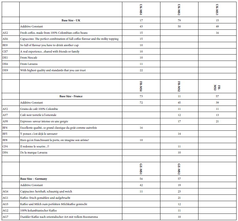
UK: One large mind-set (UK-MS2) and two smaller mind-sets (UK-MS1 and UK-MS3).
The three mind-sets show approximately the same magnitude of the additive constant (43-50)
Only one of these mind-sets shows strong performing elements, UK-MS1.
Mind-Set UK-MS3 shows only one strong performing element, AE2 Fresh coffee, made from 100% Colombian coffee beans.
France: Two large mind-sets (FR-MS1, FR-MS3) and one small mind-set (FR-MS2).
The additive constants and the strong performing elements are different.
FR-MS1 shows the highest additive constant (72), and react most strongly to descriptions of emotional experience.
FR-MS2, the smallest mind-set, shows strong responses to the elements. The base size of 11 respondents in FR-MS2 may be too low to assume FR-S2 is a ‘real’ mind-set. It may simply be the result of forcing the clustering to come up with three mind-sets.
FR-MS3 responds strongly to statements about product and features (Question A)
Germany: Only two mind-sets emerged for Germany, with the third mind-set having very respondents, and thus not shown.
All elements for Germany come from product and features (Question A).
In most Mind Genomics studies the search for mind-sets generates strongly defined, exceptionally different groups. Surprisingly, this does not seem to be the case for coffee, despite the hundreds of millions of dollars spend on advertising. It may well turn out that there is simply not enough differences among coffees to create sharply different mind-sets, based simply on description. That is, ‘coffee may just be coffee.’ There are not enough intrinsic features in coffee to drive radically different mind-sets, despite the popularity of coffee, or perhaps the underlying reason for that popularity!
Discussion
Improving Research by Reducing Bias
The approach presented here with coffee emerges with some clear patterns, the clearest of which is that the strongest performing elements in these Mind Genomics studies come from the question about product description. Although the respondents are presented by systematically varied vignettes, combinations of messages, and cannot possible ‘game’ the system, they act in a consistent manner. It is impossible to know the ‘correct’ answer when presented with a rapidly changing set of 60 vignettes. The demands on the respondent are very strong, and militate against overthinking. Yet again and again what emerges are the same types of messages. No matter how we attempt to provide additional types of information the pattern re-emerges. Only a few messages are strong.
It is important to reiterate the fact that the design in this study prevents bias. With the continuing presentation of vignettes, most respondents simply ‘turn off,’ responding automatically. The data do not suggest that the respondent down-rates the vignettes out of irritation. Yet, in many ‘exit interview’ respondents have said, by way of complaint that they felt they were guessing, that they were unable to discern a pattern which would lead to the ‘correct answer. Respondents do try to guess in these situations. The fact that they cannot discern the pattern simply means that they must react at an intuitive level, or react randomly. Yet, if respondent were to react randomly, then we would see many more elements from Questions B, C and D emerging as strong performers. They do not. The respondents do respond in a truthful manner, even if the respondents do not think so. The result may be the accuracy emerging by of averaging well-meaning ‘guesses’, with the result being the ‘correct answer’ as Surowiecki discusses in his work on the Wisdom of the Masses [21].
To summarize the differences then, the conventional questionnaire instructs the respondents to think about different aspects of the product and situation, in our case here ‘coffee.’ The respondent may be asked dozens of questions. The pattern of responses gives us an idea of how the respondent feels about coffee. The respondent may subconsciously change the responses to questions to be perceived as consistent. Indeed, the emphasis is often on answering consistently, digging into one’s own thinking to answer the question as best as possible. The interview can be perceived as a test, and there is always the worry about ‘interviewer bias,’ a concern with a history of at least three quarters of a century [22-24]. In contrast, the Mind Genomics approach creates an experiment, comprising known combinations of messages, presents these combinations, acquires the response, and estimates the driving power of each element.
A New Type of Insight
Traditional research in the world of psychology and consumer behavior has focused on attitudes towards product or services, looking at the way different ‘types’ of people respondent, or looking at how some antecedent experimental manipulation affects the response. From these data, whether through discussion, observation, or experimentation, the researcher is able to fill one more ‘hole in the literature,’ one more gap in the web of knowledge. It is through the accretion of these pieces of information, individual moments of insights, and the integrative ability of analysts with a wide scope and imagination, that the ‘story’ builds, and understanding increases.
The approach presented here, while incomplete by necessity, provides a grander, more holistic view of the topic. The study here on coffee is not only on one particular problem, one recurrent issue, but is rather an attempt to create a new type of database, multi-dimensional in nature. On the one hand we have the topic, coffee, which has been well explored on different, scientifically relevant dimensions. On the other hand, we have a product consumed around the world, which, when examined closely, lacks a deep reservoir of integrated information about the nature of people and coffee. We don’t know what messages attract people. We know that people differ, but we don’t know how they differ. Nor do we have any real idea of the co-variation of factors, such as the responsivity of individuals to coffee messages, these individuals classified by who they are, when they participate, what they hold to be important, and so forth.
The Mind Genomics paradigm creates this type of information, doing so easily and quickly. Rather than plugging ‘holes’ in the literature, closing gaps, and growing science one finding at a time, Mind Genomics becomes a holistic knowledge-development tool, creating information that is both novel and in fact occasionally fascinating.
Creating Large Databases
As emphasized throughout this paper, Mind Genomics is actually a well-constructed experiment with defied independent variables and responses. The outcome of the experiment is a database. This set of three studies shows how one can construct the database for three countries, for one product, working with respondents from each country. The studies are rapid, taking days, and cost-efficient, with estimates today as of this writing being $4-$6 per respondent for a smaller version of Mind Genomics (16 elements), with easier to find respondent. Thus, in terms of economics, the per country cost of a Mind Genomics study with 16 elements, rather than 36, is less than $1,000, low by today’s standards. Indeed, the potential exist for the enterprising consumer researcher or marketer to spend less than $100,000 to create a world-wide database of a particular product, at a particular point in time. We can only speculate about the vast increase in knowledge this database will bring, across cultures, across time, and across different mind-sets within a culture. The dream of the It! Studies, developed around the year 2000, is now immediately doable by virtually anyone (see www.BimiLeap.com and www.PVI360.com)
Acknowledgments
The author gratefully acknowledges the foundational work for Eurocrave, sponsored by Firmenich in Switzerland, with the guidance and help of Pieter Aarts of ScentTaste (Belgium), and Klaus Paulus (Germany). The late Hollis Ashman of the Understanding and Insight Group in the USA did much of the design work prior to the study, and analytics after the study.
References
- Morris J (2018) Coffee: A Global History. Reaktion Books.
- Pendergrast M (2010) Uncommon Grounds: The History of Coffee and How It Transformed Our World. Basic Books.
- Jervis SM, Lopetcharat K, Drake MA (2012) Application of ethnography and conjoint analysis to determine key consumer attributes for latte-style coffee beverages. Journal of Sensory Studies 27: 48-58.
- Samoggia A, Riedel B (2018) Coffee consumption and purchasing behavior review: Insights for further research. Appetite 129: 70-81. [crossref]
- Morris J (2013) Why espresso? Explaining changes in European coffee preferences from a production of culture perspective. European Review of History: Revue Européenne d’Histoire 20: 881-901.
- Morris J (2016) Why espresso? Explaining changes in European coffee preferences from a production of culture perspective. In Made in Europe (pp. 151-171). Routledge
- Navarini L, Cappuccio R, Suggi-Liverani F, Illy A (2004) Espresso coffee beverage: Classification of texture terms. Journal of Texture Studies 35: 525-541.
- Andorfer VA, Liebe U (2015) Do information, price, or morals influence ethical consumption? A natural field experiment and customer survey on the purchase of Fair Trade coffee. Social Science Research 52: 330-350.
- Bianco GB (2020) Climate change adaptation, coffee, and corporate social responsibility: challenges and opportunities. International Journal of Corporate Social Responsibility 5: 1-13.
- Rotaris Lucia, Danielis Romeo (2011) Willingness to pay for fair trade coffee: A conjoint analysis experiment with Italian consumers. Journal of Agricultural & Food Industrial Organization 9.
- Van Loo EJ, Caputo V, Nayga Jr RM, Seo HS, Zhang B, et al (2015) Sustainability labels on coffee: Consumer preferences, willingness-to-pay and visual attention to attributes. Ecological Economics 118: 215-225.
- Geel L, Kinnear M, De Kock HL (2005) Relating consumer preferences to sensory attributes of instant coffee. Food Quality and Preference 16: 237-244.
- Green PE, Krieger AM, Wind Y (2004) Thirty years of conjoint analysis: Reflections and prospects. In Marketing Research and Modeling: Progress and Prospects (pp. 117-139). Springer Boston, MA.
- Mead R (1990) The Design of Experiments: Statistical Principles for Practical Applications. Cambridge University Press.
- Moskowitz HR (2012) ‘Mind genomics’: The experimental, inductive science of the ordinary, and its application to aspects of food and feeding. Physiology & Behavior 107: 606-613. [crossref]
- Moskowitz HR, Gofman A, Beckley J, Ashman H (2006) Founding a new science: Mind genomics. Journal of Sensory Studies 21: 266-307.
- Foley M, Beckley J, Ashman H, Moskowitz HR (2009) The mind-set of teens towards food communications revealed by conjoint measurement and multi-food databases. Appetite 52: 554-560. [crossref]
- Rabino S, Moskowitz H, Katz R, Maier A, Paulus K, et al. (2007) Creating databases from cross-national comparisons of food mind-sets. Journal of Sensory Studies 22: 550-586.
- Gofman A, Moskowitz H (2010) Isomorphic permuted experimental designs and their application in conjoint analysis. Journal of Sensory Studies 25: 127-145.
- Likas A, Vlassi N, Verbeek JJ (2003) The global k-means clustering algorithm. Pattern Recognition 36: 451-461.
- Surowiecki J (2005) The Wisdom of Crowds. Anchor.
- Boyd Jr HW, Westfall R (1970) Interviewer bias once more revisited. Journal of Marketing Research 7: 249-253.
- Ferber R, Wales HG (1952) Detection and correction of interviewer bias. Public Opinion Quarterly 16: 107-127.
- Falkner L (2020) An exploratory study of generational coffee preferences. Falkner, Lindsey, “An Exploratory Study of Generational Coffee Preferences”. Honors College Theses.